Section 1.1: The Maclaurin Series Approach

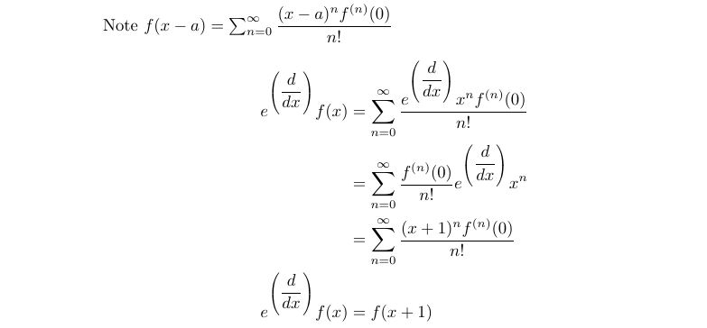
To start, we will investigate the process of raising e to the differential operator. We will utilize the Maclaurin series, a common method for exponentiation. Let’s define the Maclaurin series for e raised to the differential operator, which we will denote as D.

Next, we can multiply specific functions by e^D and observe the outcomes. A straightforward function for evaluation is e^D(e^x), as it is unique in being its own derivative.

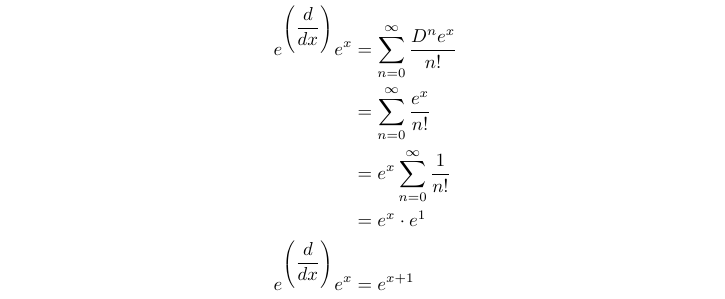
From our findings, we discover that e^D(e^x) results in a shift of the function one unit to the left. Fascinating! Next, we will explore the multiplication of e^D(x^k) where k > 0, which involves repeatedly differentiating x^k and will be instrumental in defining the multiplication of e^D by a polynomial.

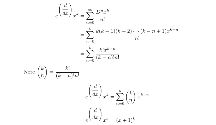
It’s intriguing that both e^D(e^x) and e^D(x^k) yield similar results, translating their respective functions leftward by one unit. Before we generalize this for any differentiable function, let’s examine another example: e^D(sin x). I have two methods for this—using repeated differentiation and leveraging complex numbers. I'll outline both approaches below, and feel free to share any additional methods you might discover!

Subsection 1.1.1: Methods for Evaluating e^D(sin x)

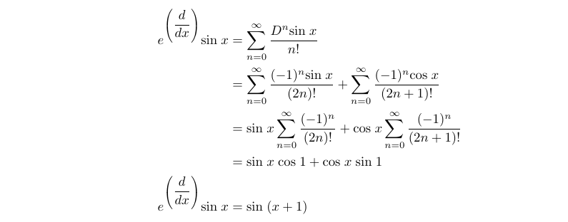
Utilizing complex numbers alongside our earlier findings with e^D(e^x) yields similar results.

Both methods indicate that sin x is translated leftward by one unit. These results and the employed techniques should enhance your comprehension when addressing the differential equations posed earlier.

Section 1.2: Generalizing the Results

Now, let’s prove that e^D effectively translates any differentiable function, f(x), to the left by one unit. We will leverage the Taylor series expansion of f(x).

After examining these examples, I wondered how similar concepts would apply to D_2 = d²/dx². This led me to significantly more complex results, which I’ll discuss later in this article. To begin, I tested e^(D_2)(e^x) using similar methods previously outlined.

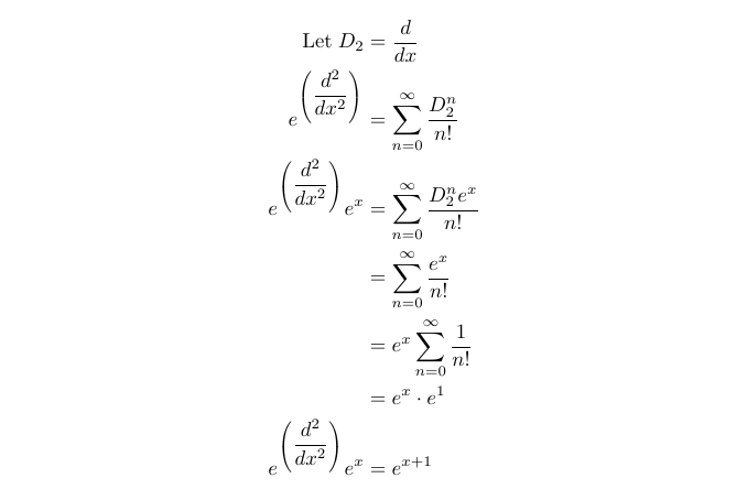
This retains the same translation as before, which makes sense due to the inherent property of e^x being its own derivative. Next, we’ll analyze e^(D_2)(sin x).

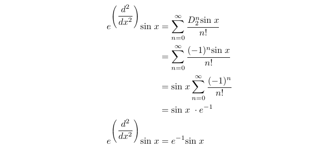
This result is unexpected. While we previously observed translations, e^(D_2)(sin x) causes a stretch in the y-direction with a scale factor of e^(-1). Thus, it appears that e^(D_2) does not produce a consistent outcome like e^D.

I also began exploring e^(D_2)(x^k), which rapidly became complicated, prompting me to consult Wolfram Alpha for assistance.

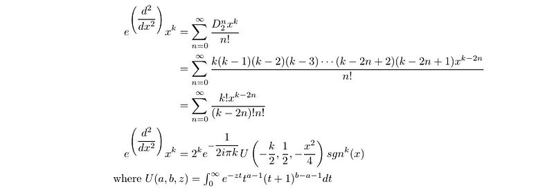
The output was not immediately clear. U(a, b, z) represents the confluent hypergeometric function of the second kind, should you wish to investigate further.

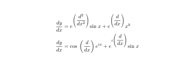
The Problems

Equipped with these methods, we can tackle the initial problems presented at the start of this article. Give them a try before we walk through the solutions utilizing the results and techniques discussed earlier.

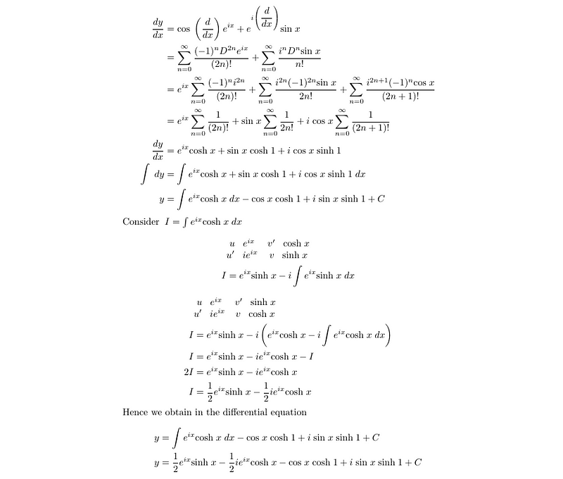
We have encountered both terms with e^D, allowing us to substitute and solve the differential equation as we normally would.

The solution was relatively straightforward once we became comfortable with the e^D components. Moving on to the next problem:

I haven’t detailed the methods for cos(D) and e^(iD), but a good starting point would be to consider their Maclaurin expansions.

In conclusion, I hope you found this exploration into these unconventional ideas engaging. Thank you for taking the time to read through this. Please feel free to share your thoughts on this concept!